Lab 1: Car Motion Lab
Title - The effect of the amount of time an object is in motion on the displacement the object travels.
Research Problem:
What is the effect of time an object is in motion on the displacement the object travels?
Variables:
Independent Variable - Time an object is in motion
Dependent Variable - Displacement the object travels
Constants - Measurement devices (meter sticks), location with each trial, stopwatch user, stopwatch software, motorized car used, and the surface on which trials were completed.
Control - There was no control in this experiment.
Dependent Variable - Displacement the object travels
Constants - Measurement devices (meter sticks), location with each trial, stopwatch user, stopwatch software, motorized car used, and the surface on which trials were completed.
Control - There was no control in this experiment.
Procedure:
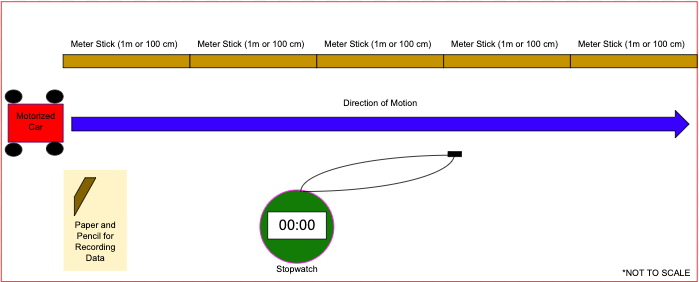
Meter sticks were placed along the ground in a straight line next to a motorized car. The car was turned on and released with its front tires even with the beginning of the first meter stick. After a predetermined amount of time, it was measured how far the car had traveled in centimeters using the meter sticks next to the car and recorded into a data table. This was repeated for four trials of different times.
Method:
Time- Independent variable, this was changed to affect the position of the car. It was measured by using a stopwatch, and this determined how long each trial was.
Position - Dependent Variable, this was changed due to the independent variable, this was measured using meter sticks and it was measured in centimeters. Since each meter stick was only one meter long, and some trials required a measurement of position greater than one meter, several meters sticks had to be used.
Velocity - calculated using the position and the time. The average velocity for each trial was by taking the change in position over the whole time, which is the final position subtracted by the initial position and dividing that value by the total time for the trial.
Diagram:
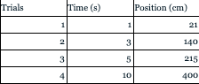
Raw Recorded Data:
Processed Data:
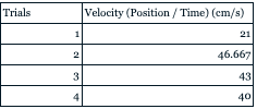
Sample Calculations and Graphical Analysis:Sample Calculations - Velocity was calculated using the values of position and time for each trial. To get the velocity of a trial, the position value has to be taken and divided by the time value. An example is trial 3, when the position is 215 cm and the time is 5 s. (215 cm / 5 s = 43 cm/s) This means the velocity of trial 3 is 43 cm/s.
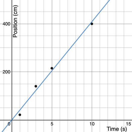
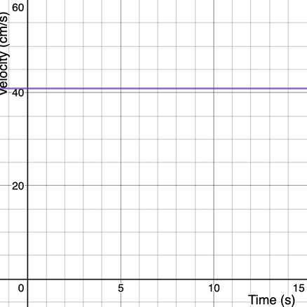
Graphical Analysis - The slope of the line of best fit on the position time graph is about 40.667 cm/s , and the y-intercept is 0 cm. This means that the equation for the line in the position time graph is (y = 40.667x). It is notable that the slope of the line has the units cm/s, which is of velocity. Also, the slope of the line is 40.667, and the y-values on all of the x-values on the velocity time graph is 40.667 (The equation for the line in the velocity time graph is y = 40.667). The slope of the line on the position time graph at a point is the velocity for that motion at that point. Since the position time graph is a straight line, then the motion will model a constant velocity, which is what is seen in the velocity time graph. |
|
Conclusions:The relationship between the amount of time an object is in motion and that object's position is linear, meaning that the velocity is constant. This is seen in data, where the velocities of 46.667 cm/s, 43 cm/s, and 40 cm/s are very similar (Excluding trial 1 as an outlier). The data from this experiment can be used to predict future trials of varying times, meaning that given a time, the position and velocity could be predicted. However, this experiment was far from perfect as there was a high level of uncertainty. One possible cause of uncertainty is the accuracy of the instruments used in the experiment including the meter sticks and the stopwatch. Another large source of uncertainty is the decision-making of the experimenters. The experimenter responsible for timing had to see when the stopwatch hit a certain value before stopping the stopwatch. Slight mistakes and imperfections could have caused major disparities in the data. A third large limitation was that the buggy did not travel in a straight line. It curved off in a direction instead of going straight, and when the only unit of measurement of position is forwards, the car gradually turning more and more as time went on will make it look slower. This is a possible reason that the velocities of trials 2, 3, and 4 begin to decrease. Ways to improve this experiment would be to use video analysis instead of a stopwatch, to improve accuracy and remove a large source of error. Another way to improve the experiment would be to use a car that travels in a straight line, so that another large source of error is removed.
|
|
Title - Mass vs. Weight Lab
Research Question:
How is mass related to weight?
Variables
Independent Variable - Mass
Dependent Variable - Weight
Constants - Measuring devices, location for each trial
Control - Planet
Dependent Variable - Weight
Constants - Measuring devices, location for each trial
Control - Planet
Procedure
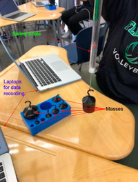
A spring scale was used to weigh the different masses used in this experiment. Masses were hanged off of the spring scale, and their weight was measured visually on the spring scale. The results were entered into a data table and graphed, and this process was completed for 10 trials.
Method
Mass - The independent variable, this was changed to affect the weight of objects in the experiment. It was pre-determined and not measured.
Weight - The dependent variable, this was affected by the mass of the object in the experiment. It was measured using a spring scale and in the units of N.
There were no further calculated values in this experiment.
Weight - The dependent variable, this was affected by the mass of the object in the experiment. It was measured using a spring scale and in the units of N.
There were no further calculated values in this experiment.
Diagram
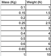
Raw Recorded Data
Sample Calculations and Graphical Analysis
|
Sample Calculations - There were no sample calculations needed for this experiment as every variable was measured and not calculated.
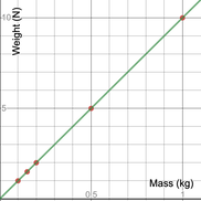
Graphical Analysis - The slope of the line through the data points is about 10 N/kg based off of the data, and the Y-intercept is 0 N. This means that the equation for the line shown on the graph is (y = 10x). It is important to note that 10 N/kg is not the actual relationship between mass and weight. The actual value is around 9.8 N/kg and the difference can be accounted to errors in the experiment. |
|
Conclusions
The relationship between the mass of an object and its weight are linear, as supported by the data collected in the experiment. As seen in the data, the slope of the line between the mass of an object and its weight has a slope of 10 N / kg. The actual value should be 9.8 N / kg, but the difference in values can be attributed to errors in the experiment. The data from this experiment can be used to predict the weight of objects with a given mass. To do this, simply take the mass in kg of an object and multiply that value by 9.8 N / kg to get the weight in N.
However, this experiment was far from perfect as there was a high level of errors within the experiment. The masses of the objects were given, and assumed to be correct, as well as the spring scale was assumed to be accurate during use as well. If these were not true then some uncertainty in the experiment could have been created. Another possible source of uncertainty in the experiment was that in order to determine the weight of a mass, the experimenters had to look at and judge at what weight the spring scale was indicating that the object weighed. This was one of the largest sources of uncertainty in the experiment and any incorrect judgement could have led to incorrect or inaccurate results.
A possible way to improve the experiment would be to use a measuring system that did not require the judgement of experimenters. A digital scale would be a possible option for weighing the masses. Another possible way to improve the experiment would be to test and verify that the masses being measured are correct and that the scales being used are accurate.
Title - Force vs. Acceleration and Mass vs. Acceleration Lab
Research Question
How do unbalanced forces affect motion?
Variables
Experiment 1:
Independent Variable - Net Force on the object
Dependent Variable - Acceleration of the object
Constant - Measuring devices and location
Control - Mass of object being pulled
Experiment 2:
Independent Variable - Mass of object being pulled
Dependent Variable - Acceleration of the object
Constant - Measuring devices and location
Control - Net Force on the object
Procedure
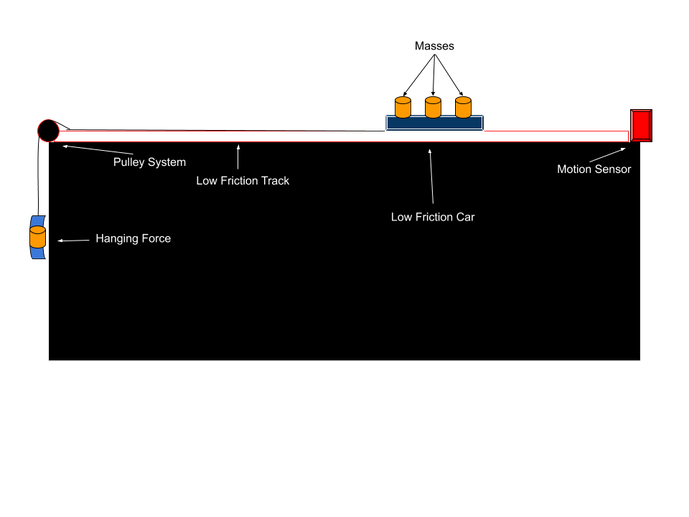
An object with weights on top of it is attached to a pulley system with a hanging mass affected by gravity and pulled along a low-friction track. The acceleration of the cart was measured using a motion detecter. After one trial was completed, then some weight on top of the object was moved to the hanging mass affected by gravity and repeated until enough trials were completed to draw accurate conclusions.
Method
Experiment 1:
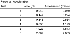
Force - Independent variable, this was changed to affect the acceleration of the object. It was measured by taking pre-determined masses and multiplying them by the acceleration due to gravity, and moving some of them from the top of the object to the hanging mass. This was measured in Newtons (N).
Acceleration - Dependent Variable, this was changed due to the independent variable. This was measured using a motion sensor in meters / second^2 (m/s/s).
Experiment 2:
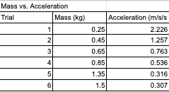
Mass - Independent variable, this was changed to affect the acceleration of the object. The masses used were pre-determined and measured in kilograms (kg).
Acceleration - Dependent Variable, this was changed due to the independent variable. This was measured using a motion sensor in meters / second^2 (m/s/s).
Force - Independent variable, this was changed to affect the acceleration of the object. It was measured by taking pre-determined masses and multiplying them by the acceleration due to gravity, and moving some of them from the top of the object to the hanging mass. This was measured in Newtons (N).
Acceleration - Dependent Variable, this was changed due to the independent variable. This was measured using a motion sensor in meters / second^2 (m/s/s).
Experiment 2:
Mass - Independent variable, this was changed to affect the acceleration of the object. The masses used were pre-determined and measured in kilograms (kg).
Acceleration - Dependent Variable, this was changed due to the independent variable. This was measured using a motion sensor in meters / second^2 (m/s/s).
Diagram
Raw Recorded Data
Sample Calculations and Graphical Analysis
|
Sample Calculations - There were no sample calculations needed for this experiment as every variable was measured and not calculated.
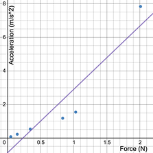
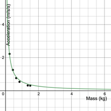
Graphical Analysis - On the first graph it can be seen that there is a linear relationship between the unbalanced net force acting on object and the acceleration of that object. This means that as the force increases, the acceleration will also increase. The y-intercept of the graph is a negative number, which is incorrect because if there is no net force, there cannot be an acceleration on an object, including negative accelerations. The y-intercept should be zero, and the difference can be accounted for errors in the experiment. On the second graph it can be seen that there is an inverse relationship between mass and acceleration of an object. This means that if the mass of an object is increased, then the acceleration of that object will decrease. However, a change in mass when the mass is very small will impact the acceleration more than the same change would with a larger mass. This means that the relationship between the mass of an object and its acceleration is not linear. There is no y-intercept on this graph as there is a vertical asymptote at x = 0. |
|
Conclusions
The relationship between force and acceleration is linear as seen on the first graph in the Sample Calculations and Graphical Analysis section. This conclusion is supported by Newton's second law, which states that the net force of an object is equal to its mass times its acceleration (Fnet = ma). Since the mass was constant in this part of the experiment, then the net force of an object will be equal to the acceleration times some constant value, which is a linear relationship. In the second part of the experiment it was discovered that the mass is inversely related to the acceleration of the object. This means that as mass increased, then the acceleration decreased. This is also supported by Newton's second law, as force was held constant in this experiment. The equation can be rearranged to Fnet * a = m. This shows that if mass increases, then acceleration has to decrease, if Fnet is constant.
However, this experiment was far from perfect as there was a high level of errors within the experiment. The masses of the objects were given, and assumed to be correct, as well as the accuracy of the scale used to measure materials in the experiment like the low friction car. Another possible source of error in the experiment was the accuracy of the motion sensor and the software used to determine the raw data of the experiment. The software had to use a position time graph to then find a velocity time graph, and then had to use the velocity time graph to create an acceleration time graph. These transitions could have created a large amount of uncertainty in the experiment and produced inaccurate results.
One possible way to improve the accuracy of the experiment is to use video analysis to track the motion of the low friction car. It would take a much larger amount of time to complete, but would yield more accurate results than using the motion sensor. Another possible way to improve the experiment would be to test and verify that the masses being measured are correct and that the scales being used are accurate.
